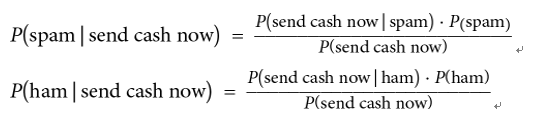
For example, imagine we have an email with three words: send cash now. We’ll use naïve Bayes to classify the email as either being spam or ham:
We are concerned with the difference of these two numbers. We can use the following criteria to classify any single text sample:
- If P(spam | send cash now) is larger than P(ham | send cash now), then we will classify the text as spam
- If P(ham | send cash now) is larger than P(spam | send cash now), then we will label the text ham
Because both equations have P (send money now) in the denominator, we can ignore them. So, now we are concerned with the following:

Let’s work out the numbers in this equation:
- P(spam) = 0.134063
- P(ham) = 0.865937
- P(send cash now | spam) = ???
- P(send cash now | ham) = ???
The final two likelihoods might seem like they would not be so difficult to calculate. All we have to do is count the number of spam messages that include the send money, right?
Now, phrase and divide that by the total number of spam messages:
df.msg = df.msg.apply(lambda x:x.lower())
# make all strings lower case so we can search easier
df[df.msg.str.contains(‘send cash now’)].shape # == (0, 2)
Oh no! There are none! There are literally zero texts with the exact phrase send cash now. The hidden problem here is that this phrase is very specific, and we can’t assume that we will have enough data in the world to have seen this exact phrase many times before.
Instead, we can make a naïve assumption in our Bayes’ theorem. If we assume that the features (words) are conditionally independent (meaning that no word affects the existence of another word), then we can rewrite the formula:

And here’s what it looks like done in Python:
spams = df[df.label == ‘spam’]
for word in [‘send’, ‘cash’, ‘now’]:
print( word, spams[spams.msg.str.contains(word)].shape[0] / float(spams.shape[0]))
Printing out the conditional probabilities yields:
- P(send|spam) = 0.096
- P(cash|spam) = 0.091
- P(now|spam) = 0.280
With this, we can calculate the following:

Repeating the same procedure for ham gives us the following:
- P(send|ham) = 0.03
- P(cash|ham) = 0.003
- P(now|ham) = 0.109
The fact that these numbers are both very low is not as important as the fact that the spam probability is much larger than the ham calculation. If we do the calculations, we get that the send cash now probability for spam is 38 times bigger than for spam! Doing this means that we can classify send cash now as spam! Simple, right?
Let’s use Python to implement a naïve Bayes classifier without having to do all of these calculations ourselves.
First, let’s revisit the count vectorizer in scikit-learn, which turns text into numerical data for us. Let’s assume that we will train on three documents (sentences), in the following code snippet:
# simple count vectorizer example
from sklearn.feature_extraction.text import CountVectorizer # start with a simple example
train_simple = [‘call you tonight’,
‘Call me a cab’,
‘please call me…
PLEASE 44!’]
# learn the ‘vocabulary’ of the training data vect = CountVectorizer()
train_simple_dtm = vect.fit_transform(train_simple) pd.DataFrame(train_simple_dtm.toarray(), columns=vect.get_feature_names())
Figure 11.3 demonstrates the feature vectors learned from our dataset:
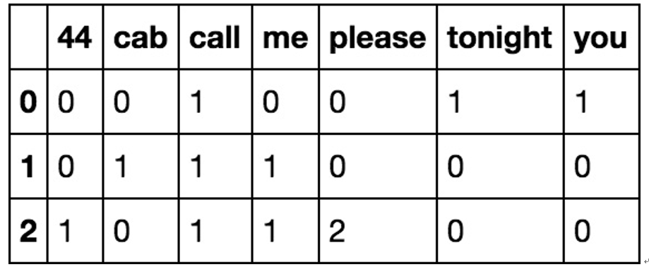
Figure 11.3 – The first five rows of our SMS dataset after breaking up each text into a count of unique words